Regression

This document shows how to use R/Studio to create output that is similar to that shown in Lock^5 (3^\text{rd} Ed.).

Section 9.1

In this section we look at inference for slope and correlation. To do so we need to import some data. We start by looking at the cricket chirp data from the book’s data repository.

Code

  ### Read the CSV file
  crickets = read.csv("http://facweb1.redlands.edu/fac/jim_bentley/Data/Lock5Ed3/Lock5Data3eCSV/CricketChirps.csv")
  ### See what is in the "crickets" dataframe to see if it worked
  crickets

  Temperature Chirps
1        54.5     81
2        59.5     97
3        63.5    103
4        67.5    123
5        72.0    150
6        78.5    182
7        83.0    195

The above seven observations look to be the same as those in the original CSV file.

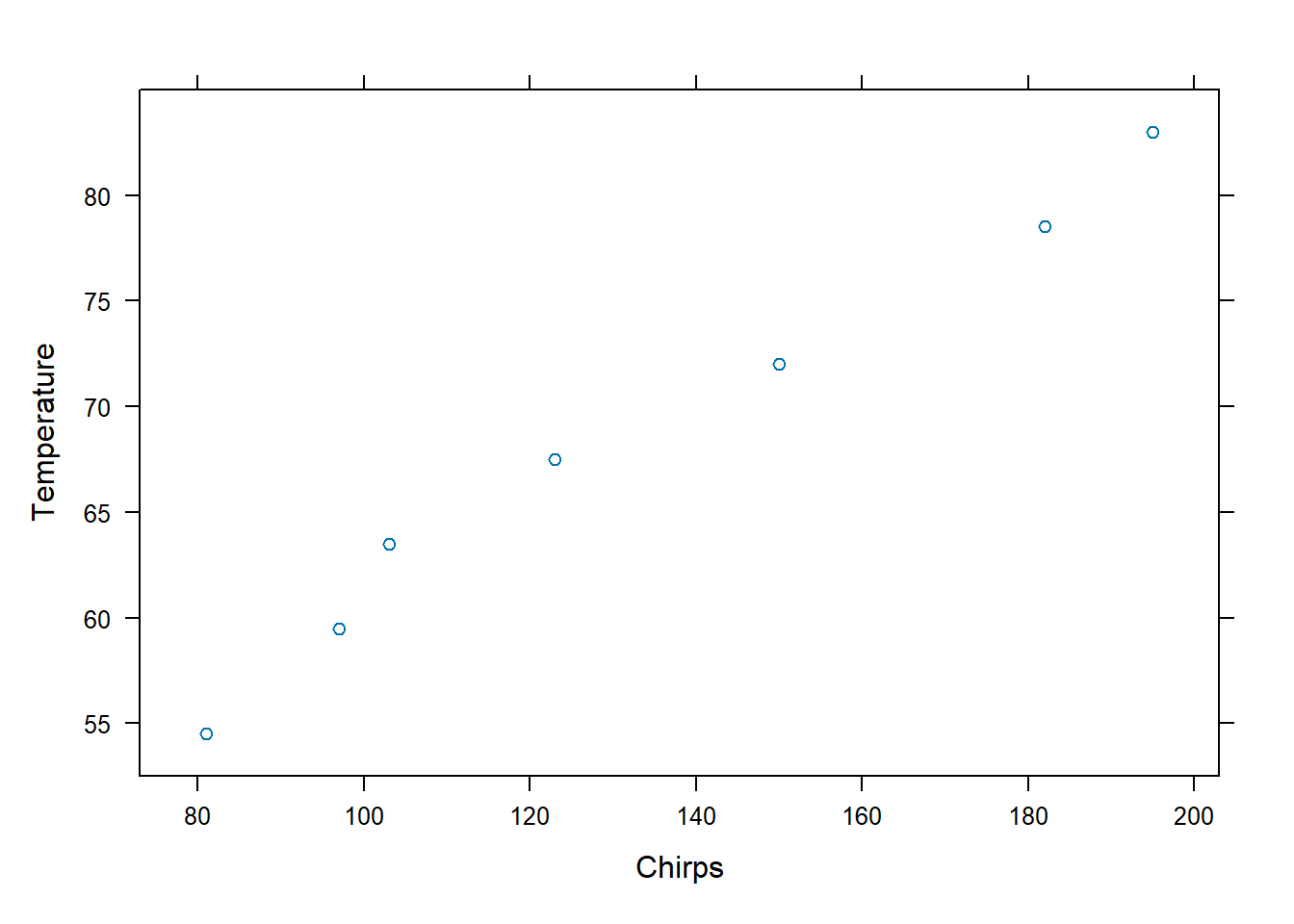
Suppose that we are interested in predicting Temperature from the number of Chirps that the crickets generate. We can plot the data to see if the relationship appears to be linear.

Code

  ### Load the lattice package to make plotting easy
  library(lattice)
  ### Now plot the points.  Note the use of ~ instead of = in the formula
  xyplot(Temperature ~ Chirps, data=crickets)

Although there are not many points, the relationship appears to be fairly linear. R makes getting the regression equation easy.

Code

  ### Get the regression equation by fitting the linear model (lm)
  lm(Temperature ~ Chirps, data=crickets)

Call:
lm(formula = Temperature ~ Chirps, data = crickets)

Coefficients:
(Intercept)       Chirps  
    37.6786       0.2307  

Code

  ### Save the linear model for later use
  crickets.lm = lm(Temperature ~ Chirps, data=crickets)
  ### Check to see if it was saved
  crickets.lm

Call:
lm(formula = Temperature ~ Chirps, data = crickets)

Coefficients:
(Intercept)       Chirps  
    37.6786       0.2307  

Code

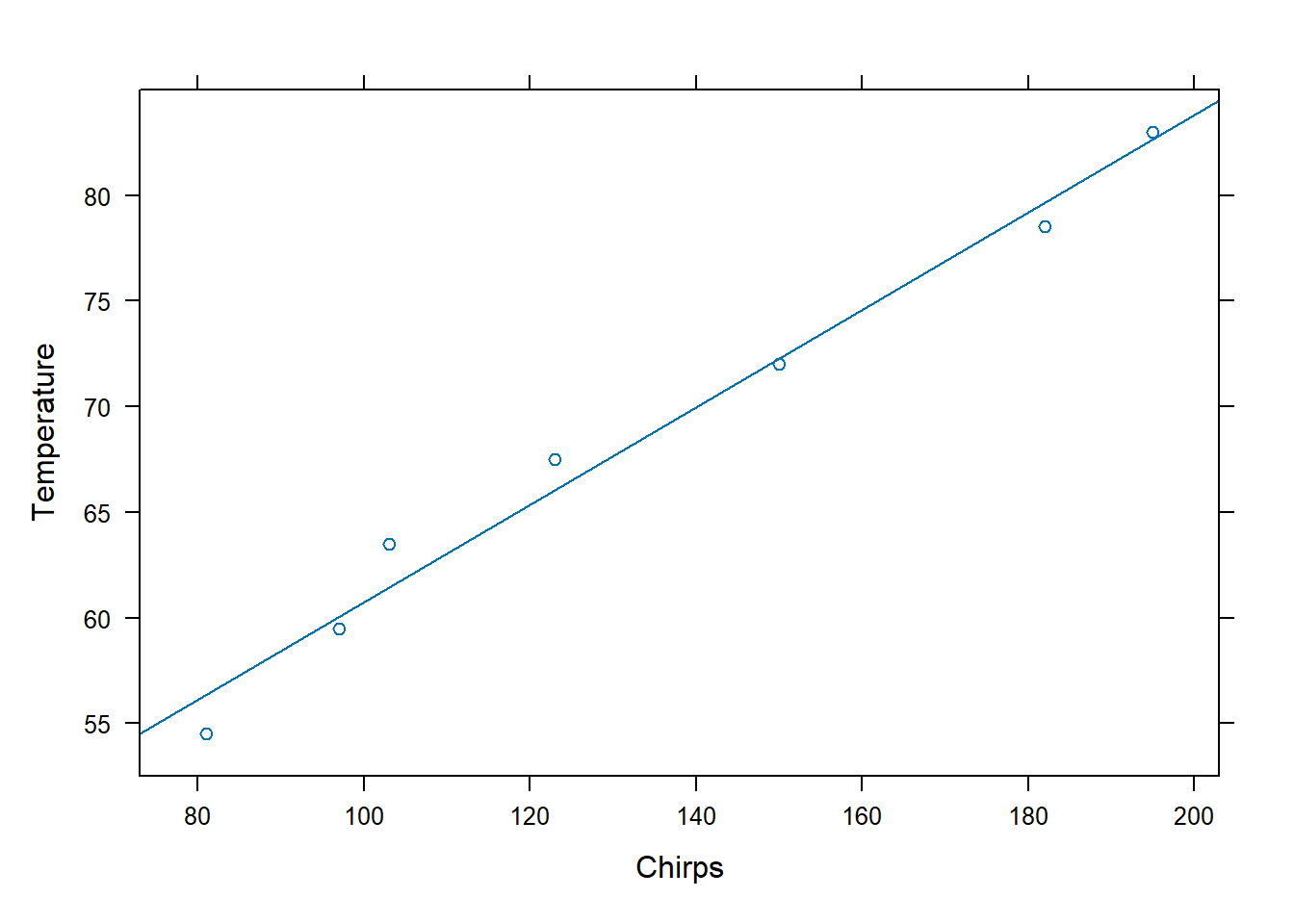
  ### Plot the points and the regression line using p and r for points and regression
  xyplot(Temperature ~ Chirps, data=crickets, type=c("p","r"))

The model is Temperature = 37.677 + 0.231(Chirps). What is a 95% confidence interval for \beta_1? Is the slope significantly different from zero? That is, does Chirps add anything to the guess of Temperature? We can let R compute the standard error and t-value that are needed to test H_0: \beta_1 = 0 versus H_A: \beta_1 \ne 0.

Code

  ### Check that the linear model fitted above is still around
  crickets.lm

Call:
lm(formula = Temperature ~ Chirps, data = crickets)

Coefficients:
(Intercept)       Chirps  
    37.6786       0.2307  

Code

  ### Now get a summary that contains the coefficients and standard errors
  summary(crickets.lm)

Call:
lm(formula = Temperature ~ Chirps, data = crickets)

Residuals:
      1       2       3       4       5       6       7 
-1.8625 -0.5532  2.0628  1.4495 -0.2785 -1.1598  0.3416 

Coefficients:
            Estimate Std. Error t value Pr(>|t|)    
(Intercept) 37.67858    1.97817   19.05 7.35e-06 ***
Chirps       0.23067    0.01423   16.21 1.63e-05 ***
---
Signif. codes:  0 '***' 0.001 '**' 0.01 '*' 0.05 '.' 0.1 ' ' 1

Residual standard error: 1.528 on 5 degrees of freedom
Multiple R-squared:  0.9813,    Adjusted R-squared:  0.9776 
F-statistic: 262.9 on 1 and 5 DF,  p-value: 1.626e-05

Note that the line that starts with Chirps contains an estimate (0.23067) and a standard error (0.01423). These values can be used to create a confidence interval for \beta_1. We note that the degrees of freedom for the t-distribution are df = 7-2 = 5. We now compute a 95% confidence interval using b_1 \pm t^*_{n-2} \cdot SE

Code

  ### Compute t-star for 5%/2 = 2.5% to the right with df=5
  qt(0.025, 5, lower.tail=FALSE)

[1] 2.570582

Code

  ### Compute the endpoints using the information found above
  0.23067 - 2.57058 * 0.01423

[1] 0.1940906

Code

  0.23067 + 2.57058 * 0.01423

[1] 0.2672494

So, it appears that we can be 95% sure that the slope of the population model, \beta_1, is in the interval (0.194, 0.267). That is, we are 95% sure that the slope of the model to predict temperature from cricket chirp rate is between 0.194 and 0.267 degrees F per chirp.

We now test to see if \beta_1 is equal to zero.

Code

  ### Compute t and the degrees of freedom
  (0.23067-0)/0.01423

[1] 16.21012

Code

  7-2

[1] 5

Code

  ### Get the p-value for a two-sided alternative using the right tail of the t distribution for t = 16.2101
  pt(16.2101, 5 , lower.tail=FALSE)*2

[1] 1.628652e-05

From the above we see that the t-value is t = (0.23067 - 0)/0.01423 = 16.2101 which has df = 7-2 = 5 degrees of freedom. This compares well with R’s value of 16.21.

Using either StatKey or R we can find the p-value by finding the area above 16.21 when there are 5 degrees of freedom. Above we see that R computes the p-value as 0.0000163. This is the same p-value presented in the table under Pr(>|t|) and indicates that We have very strong evidence that slope is different from zero, and that temperature is related to cricket chirp rates.

R also computes the correlation between two variables.

Code

  ### Compute the correlation between temperature and chirps
  cor(crickets$Temperature, crickets$Chirps)

[1] 0.9906249

Code

  ### Cheat and find the correlation between all variables in the dataframe
  cor(crickets)

            Temperature    Chirps
Temperature   1.0000000 0.9906249
Chirps        0.9906249 1.0000000

To test H_0: \rho = 0 versus H_A: \rho \ne 0 we compute the t statistic t = \frac{r - 0}{\sqrt{\frac{1 - r^2}{n-2}}} = \frac{r\sqrt{n-2}}{\sqrt{1-r^2}} which has an approximate t-distribution with n-2 degrees of freedom. For the cricket data this is

Code

  ### Compute the sample correlation, r
  cor(crickets$Temperature, crickets$Chirps)

[1] 0.9906249

Code

  ### Compute t
  (0.9906249*sqrt(7-2))/sqrt(1-0.99062^2)

[1] 16.21058

This value is the same (within rounding) as the t-statistic computed using the slope. The p-value will be the same as well. R computes these values for us more easily using the cor.test function.

Code

  ### Use cor.test to get the t-stat and p-value
  cor.test(crickets$Temperature, crickets$Chirps)

    Pearson's product-moment correlation

data:  crickets$Temperature and crickets$Chirps
t = 16.215, df = 5, p-value = 1.626e-05
alternative hypothesis: true correlation is not equal to 0
95 percent confidence interval:
 0.9352953 0.9986740
sample estimates:
      cor 
0.9906249 

It is easy to get the coefficient of determination, R^2 = r^2, using R.

Code

  ### Find the correlation, r
  r = cor(crickets$Temperature, crickets$Chirps)
  r

[1] 0.9906249

Code

  ### Now square it to get R-squared
  r^2

[1] 0.9813377

For the cricket data, Chirps explains about 98.1% of the variability in Temperature via the regression line. Stated another way, the proportion of variability in temperature that is explained by the model based on chirp rate is about 0.981. Note that this value corresponds to the “Multiple R-squared” value from the summary table above.

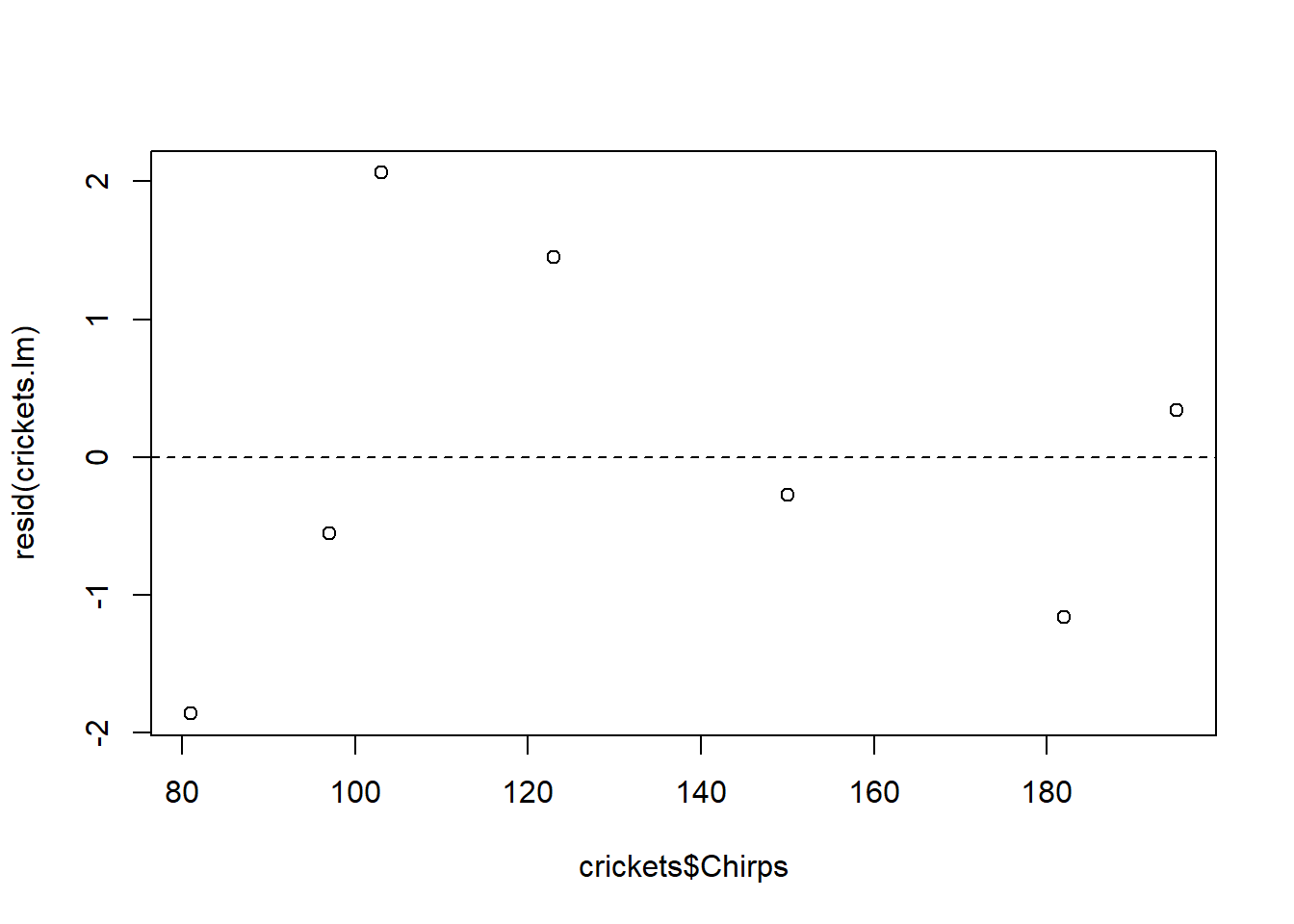
We should check the residuals to make sure that the assumptions that are made when fitting a regression model have been satisfied. Plots of the residuals help with this.

Code

  ### Replot the data with the regression line
  xyplot(Temperature ~ Chirps, data=crickets, type=c("p","r"))

Code

  ### Plot the residuals against the explanatory variable
  plot(crickets$Chirps, resid(crickets.lm))
  abline(h=0, lty=2)

Code

  ### Plot the normal probability plot
  qqnorm(resid(crickets.lm))
  qqline(resid(crickets.lm))

With only seven observations it is difficult to say that the assumptions have not been satisfied. There do not appear to be any serious outliers or influential observations. We also do not see any obvious departure from normality.